MIDS User Guide

The Model Inference and Differencing Suite (MIDS) can be used to infer software behavior models from existing software components. The models provide insight into the current software behavior. They can also be used to bootstrap the introduction of Model-Driven Engineering (MDE), reducing the need for laborious and error-prone manual modelling. Furthermore, the software behavior (models) of different software versions can be compared to find differences, detect regressions and reduce risks for software changes, such as patches and redesigns. MIDS allows performing all this in a single integrated environment. The ultimate goal is to improve the efficiency of software development and re-engineering, and reduce risks for software evolution.

MIDS can be downloaded at https://tno.github.io/MIDS/.

The documentation in this user manual is split into several chapters, together explaining how to work with MIDS:

MIDS concepts: Introduction to the concepts that are used within MIDS and a first overview of the tool.
Importing a measurement: Discusses Timed Message Sequence Charts (TMSCs), the input required for MIDS.
Constructive Model Inference: Discusses Constructive Model Inference (CMI) to infer software behavior (models).
Change impact analysis: Discusses change impact analysis by comparing software behaviors of different software versions.
Release Notes: The release notes of the various MIDS releases.

The User Guide can also be downloaded as a PDF from here.

1. Introduction

1.1. MIDS concepts

Many complex cyber-physical systems have software with a component-based service-oriented architecture. Together the components implement the full functionality of the system. Some components are services that provide a service to one or more other components. The different components are connected through interfaces, over which they communicate which each other.

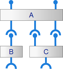
To fully realize the vision of a component-based architecture, clear contracts for the interfaces between components must be established. The contracts typically consist of several parts. The part that is commonly available is the syntax of the interactions, the function or method signatures, including names, arguments and types. This is often specified in e.g. header files (such as for C/C++) or in an interface description language (IDL). However, the behavioral protocol of allowed functional interactions is just as important, and is often not available. The protocol can be extended to include data relations (the effect of function parameters and return values). Finally, other extensions such as timing and resource usage can be included, to completely specify a contract.

Using behavioral models of the components, the behavior of different components can be analyzed, compared, optimized, etc. Since strict interfaces are defined, the environment of the component can be abstracted away. Analysis can then be restricted to the externally observable behavior of the component over the interfaces via which it communicates. By using a separate model for each component, the behavior of each component can be analyzed and qualified in isolation. This compositionality allows individual teams within a company to work on a single component, without the need to have models of all other components. Also, compositionality makes it feasible to check certain properties, for which it is not computationally infeasible to check them on a whole system at once. By restricting analysis to the behavior of the component over the interfaces via which it communicates, also (many of the) internal details of the implementation of the component can be abstracted away.

The software for components can be developed using Model-Based Engineering (MBE), also called Model-Driven Engineering (MDE). For components developed using formal MDE tooling, interface models are available that formally describe the protocol of the interface, to which clients and servers must adhere. Design models may also be available that formally define the implementation (or realization) of the component, including all internal details. However, in most companies, not all components are not (yet) developed using the MDE methodology. To be able to analyze components developed using traditional software engineering methodologies, models must be obtained for the behavior of such components.

The vision of MIDS is to provide an environment that facilitates (software) domain experts to obtain such models, and work with them. More concretely, MIDS allows to automatically infer models from existing software, using Constructive Model Inference (CMI). CMI uses dynamic information obtained from a running system, in the form of execution traces. By combining resulting behavioral models, as well as by injecting domain knowledge, a more complete behavioral model can be obtained.

The analyses that can be performed on the behavioral models can be applied for various uses, including but not limited to:

Legacy replacement (or 'drop-in' replacement), where the implementation of a component is replaced by a new implementation. The new implementation must be compatible with the legacy implementation, and must still communicate with its clients and servers in a proper way. The model can also be used to compare the behavior of the legacy and new implementations, to see whether or not they have the same behavior, and if not, where they differ. This helps to reduce risks for redesigns.
A behavioral model of an existing system can give insight into the normal and abnormal behavior of a component.
The software before and after a software change (e.g. patch, redesign) can be compared to ensure only the expected changes were made and no regressions were introduced. This reduces risks for software changes.
Information on behavior observed during tests can be compared against behavior observed during production, to find out whether all production behavior is covered by tests. In case not all production behavior is covered by tests, the information can help to provide information about what tests to add.
Information on behavior exposed by a component can be compared against behavior observed during test or production runs, to see what implemented behavior is never used during testing or in practice.
Erroneous behavior (e.g. a failing test case) can be compared with correct behavior (e.g. preceding successful runs of the same test suite), to determine where exactly deviations occur, to analyze regressions and flaky tests.

1.2. MIDS tool

The MIDS IDE is an Integrated Development Environment (IDE) based on the Eclipse IDE. The MIDS IDE also comes bundled with command line scripts. For more information, as well as download links, see https://tno.github.io/MIDS/.

Within the MIDS IDE, the files to work with are part of a project. The available projects are shown in the Project Explorer.

MIDS provides its own Eclipse perspective configuring all recommended views to be visible. This perspective is set by default, but can also be manually set as described in the Eclipse documentation.

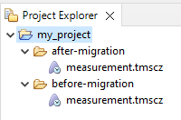
Each project is simply a directory on the hard disk, and can be expanded to show the files and directories it contains.

One way to work with files and directories is to right click on them, showing a menu with various commands.

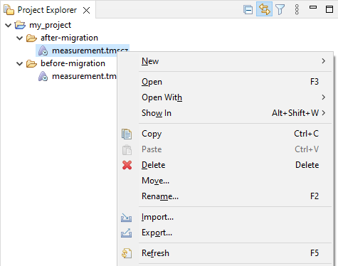
For instance, it is possible to remove or rename a file, create a new file in a directory, etc. Most of this is standard Eclipse functionality. MIDS does provide some additional commands, specific to the functionality it provides. Such commands are explained in more detail in other parts of this user guide.

Another way to work with files is to open them in an editor. By double clicking a file, it is opened in the default editor that is associated with that file. The specific functionality available in MIDS is explained in other parts of this user guide.

2. Importing a measurement

MIDS provides Constructive Model Inference to automatically infer models from execution traces. CMI works on execution traces, in the form of Timed Message Sequence Charts (TMSCs). The details of how to produce a TMSC from your company’s proprietary logging format, are beyond the scope of this documentation.

3. Constructive Model Inference

Passive learning allows inferring models from (execution) traces. If execution traces are available, access to the actual system is not required. Since the inputs for passive learning are execution traces, the learned models are models of the executed behavior. To obtain a model of the complete behavior of a component or system, one needs traces that cover all different parts of the system behavior. For instance, one could combine traces from normal execution scenarios with traces from test cases that cover exceptional behavior.

MIDS supports the Constructive Model Inference (CMI) method of learning models. Contrary to existing heuristic-based approaches, this method uses domain knowledge about the system, e.g. its architecture, communication patterns, middleware, deployment and conventions. This knowledge is used to interpret execution traces and construct models that capture one’s intuition of the system, and can be easily understood and relied upon, without configuring complex parameters. Models can be constructed at different levels of abstraction, e.g. system, component, and interface models.

The inferred models provide valuable insight into the current software behavior. They can can be used to bootstrap the transition to Model-Driven Engineering (MDE). The insights they provide are also useful when making changes to the software, as it is difficult to make changes to software without understand how it behaves. Furthermore, after you have made your changes, the models can be automatically compared, allowing for change impact analysis.

3.1. Event naming scheme

For every start/end of a function call on a component, we have an event in our models. The events are named using our naming scheme. The following is an overview of the scheme:

Component identity Method Type of call/handler Return Other side

Component identity	Method	Type of call/handler	Return	Other side
<component identity> `.`	<interface name> `__` <function name> `_`	`_blk`	none (function start)	none (internal event)
	`_lib`	`_ret` (function end)	`__` <component identity>
`_req`
`_wait`
`_fcn`
`_fcncb`
`_sync`
`_async`
`_arslt`
`_evtsub`
`_evtsubh`
`_evtunsub`
`_evtunsubh`
`_evt`
`_evtcb`
`_trig`
`_trigh`
`_call`
`_handler`
`_unkn`

<component identity> .

<interface name> __ <function name> _

_blk

none (function start)

none (internal event)

_lib

_ret (function end)

__ <component identity>

_req

_wait

_fcn

_fcncb

_sync

_async

_arslt

_evtsub

_evtsubh

_evtunsub

_evtunsubh

_evt

_evtcb

_trig

_trigh

_call

_handler

_unkn

The name always starts with the name of the first component involved. This is the component that declares the event. It represents one of two options:

The component on which the internal event occurs.
The source component of a communicating event.

The name of the interface and function are added to uniquely know the identity of the software function. They are separated by a double underscore. The type of call or handler is added, after an additional underscore to separate it from the function name. The following options are present:

`_blk`	A blocking call.
`_lib`	A library call.
`_req`	A request call.
`_wait`	A wait call.
`_fcn`	An FCN call.
`_fcncb`	An FCN callback handler.
`_sync`	A synchronous handler.
`_async`	An asynchronous handler.
`_arslt`	An asynchronous result call for an asynchronous handler.
`_evtsub`	An event subscription call.
`_evtsubh`	An event subscription handler.
`_evtunsub`	An event unsubscription call.
`_evtunsubh`	An event unsubscription handler.
`_evt`	An event raise call.
`_evtcb`	An event callback handler.
`_trig`	A trigger call.
`_trigh`	A trigger handler.
`_call`	An abstract call.
`_handler`	An abstract handler.
`_unkn`	An unknown call/handler, e.g. due to this host being untraced.

For every function call there is the start and end of that function call. The end of a function call gets an additional _ret (for “return”) added to its name. In case the event represents communication to another component, the following applies:

The type of the other side and _ret if applicable, are also added for the other side.
The identity of the component on the other side is added, if it does not involve communication to itself (e.g. multiple servers deployed on a single OS process or thread). It is separated from the event type by a double underscore.
If two runtime components (OS processes/threads) are involved, the order is chronological. That is, the first component starts the communication. The first type and _ret apply to that component. The second type and _ret apply to the receiving component, the second component identity is the receiving component. The name reads from left to right chronologically, as: “this component calls this function in this way and it is handled in this way by the other component”.

For two events connected by a dependency, the CIF event will be the same for both events, to ensure they synchronize. E.g. Component1.SomeInterface__some_function__blk_sync__Component2.

For more information about the communication patterns, see this scientific paper (primarily Section 4.1).

3.2. Inferring models

In order to perform CMI, you can use the mids-cmi command-line tool.

The CMI tool has a number of configurable options. The tool provides a list of available options if used with the -h or -help option.

The first parameter configures which trace data is used to infer models. Providing the input path is required to perform CMI.

Input file (-i or -input): Constructive Model Inference takes a TMSC, i.e. a .tmscz file, as input.

This means the basic command to run the CMI tool is mids-cmi -i some-folder/input.tmscz or mids-cmi -input some-folder/input.tmscz. By default, the CMI tool will put the resulting models in a folder called cmi next to the input TMSC file. If such a folder does not exist, it will be created by the tool.

To customize the CMI process and the output, a number of other options are available. The other available options are:

Output folder (-o or -output)

The output of CMI is stored in the location specified. If the provided path does not describe an existing folder, a new folder will be created. Specify this option to override the default output folder location.

Save yEd diagrams (-y or -yed)

By default, only CIF files are written for the inferred models. If the Save yEd diagrams option is enabled, in addition to CIF models, yEd visualizations of the final models are also generated. These can be used to inspect the models, to get insight into the software behavior. yEd can be downloaded at https://www.yworks.com/products/yed.

Infer protocol between two components (-p or -protocol)

The output of model inference is either component models or a single protocol model. By default, one or more component models are created. If this option is enabled, the output is instead a single protocol model representing communication between a pair of components. If protocol inference is chosen, two components have to be selected as communicating parties in the protocol. Components can be selected by providing the two component names as argument of the option, separated by a comma. Note that computing the protocol can be very memory-intensive and time-consuming. Protocol models are always prefix-closed.

Additional protocol scope components (-ps or -protocolscope)

If the option to infer a protocol is chosen, extra context components can be added to the scope of the protocol computation, as a comma separated list of component names. These additional components will not be directly present in the final protocol, but will be taken into account to determine the allowed order of events in the protocol. Note that adding extra components increases the memory and time requirements of the computation. If component models are being inferred rather than a protocol, this option will be ignored.

Do not convert events on untraced components to synchronous functions (-u or -no-untraced-synchronous)

By default for each component that is untraced, superfluous events and dependencies that link the start and end of a synchronous function are removed. This reduces the size of the models makes further analysis easier. If combining the dependency information to form a single event is undesired, this option can be used to disable it.

Do not synchronize dependent (-d or -no-sync-dependent)

As part of the transformation of TMSC events to CIF events, the component initiating the event has to be identified. By default, for communicating events information from the source and target of the corresponding dependency is combined into a single CIF event. Otherwise, only local information is used for the CIF event. If this behavior is undesired, this option can be used to disable it. Note that unless you want to use explicit middleware models, disabling the synchronization is not recommended.

Save single model (-s or -single-model)

By default, each component model created by Constructive Model Inference is stored in a separate CIF model. If this option is selected, a single CIF model containing all components is created instead. When inferring a protocol model rather than component models, this option is ignored. Additionally, if the option to generate yEd diagrams is enabled, this option has no effect on that, as always only a single diagram is constructed for all components.

Component exclusion regex (-ce or -component-exclusion)

Component inclusion regex (-ci or -component-inclusion)

Filtering can be applied by including and/or excluding components based on their name. A filter consists of a Java regular expression provided as argument to the option, which will be matched against all component names. For a component exclusion filter, components matching the pattern will be rejected. For a component inclusion filter, components not matching the pattern will be rejected. Models for components removed by filtering are discarded and will not be processed further or stored. There can be at most one exclusion filter and one inclusion filter defined.

Perform post-processing operation (-c or -post-processing)

Furthermore, post-processing operations can be applied to the inferred models. Each operation added will be applied to the models in the order they are listed on the command line. Each operation can require a certain precondition or result in a certain postcondition with regard to the existence or lack of data and/or tau events in the inferred models. If a precondition for an operation is not satisfied, the operation may fail, e.g. when an operation requires tau events to be present, but they are not present. Operations may also eliminate certain concepts automatically, if they don’t support them. E.g. data may be eliminated if an operation only works for models without data. Note that as part of post-processing the number of models may increase or decrease.

To add a post-processing operation, its name and any required arguments must be supplied. It is possible to add multiple operations by supplying the option multiple times. For most operations, it is possible to configure to which components they are applied with filtering. Filtering is defined by adding <filter-mode,filter-pattern> before the operation name. Filter mode has to be either inclusion or exclusion, and the filter-pattern has to be a Java regular expression for matching component names. During processing, each component name is matched against the filter-pattern provided. If the filter-mode is inclusion, the operation is applied to components that match the pattern, and not applied to those that do not. If the filter-mode is exclusion, the filtering is reversed. As a basic example, if the argument ModifyRepetitions(data,0,0,false,0) is supplied, the ModifyRepetitions operation is applied to all models with the provided arguments. If <inclusion,ABC.*>ModifyRepetitions(data,0,0,false,0) is supplied instead, the operation is only applied to the components with names that fit the pattern ABC.*, i.e. that start with ABC. In contrast, if <exclusion,ABC.*>ModifyRepetitions(data,0,0,false,0) is supplied, the operation is only applied to components with names that do not fit the pattern.

The following post-processing operations are available:

AddAsynchronousPatternConstraints

Add constraints that enforce that asynchronous replies happen after the corresponding request, and that each asynchronous request results in a corresponding reply before the same request is made again. Also allows such constraints to be visualized in the yEd diagrams. This operation requires no configuration. This operation can be selectively applied based on filtering.

ExcludeInternalTransitions

Remove transitions from the models that do not represent a communication between two components. For the purpose of this transformation, events on transitions to and from the initial state (the start and end of service fragments) will always be considered communication. Note that this means transitions with those events will not be removed, even elsewhere in the state machine. This operation requires no configuration. This operation can be selectively applied based on filtering.

FilterClientServerInteractions(component1, component2)

Remove all service fragments that are not involved in communication between two specified components. The operation has to be configured with two components, which should communicate for the output to be useful. This operation can not be selectively applied based on filtering.

HideActions(pattern)

Remove all actions fitting a given Java regular expression pattern from the models. This operation has to be configured with a pattern to define actions that should be hidden. In order to keep models consistent, events on transitions to and from the initial state (the start and end of service fragments) will never be hidden. Note that this means transitions with those events will not be removed, even elsewhere in the state machine. This operation can be selectively applied based on filtering.

InjectDomainKnowledge(operator, model-path)

Combine inferred models with a domain knowledge model. This operation can be configured by providing a path to the domain knowledge model, which must be a CIF model, and selecting the operator that will be used to add the domain knowledge to the inferred models.

Injecting unsuitable domain knowledge can cause following operations to malfunction and fail.

The available operations are intersection, union, difference-left, difference-right, exclusive-or and parallel-composition. Suppose we have the domain knowledge model /domain.cif:

InjectDomainKnowledge(intersection,some-folder/domain.cif) would compute the behavior present in both the CMI model and the domain knowledge model.
InjectDomainKnowledge(union,some-folder/domain.cif) would compute the behavior present in either the CMI model or the domain knowledge model, or in both.
InjectDomainKnowledge(difference-left,some-folder/domain.cif) would compute the behavior present in the domain knowledge model, but not in the CMI model.
InjectDomainKnowledge(difference-right,some-folder/domain.cif) would compute the behavior present in the CMI model, but not in the domain knowledge model.
InjectDomainKnowledge(exclusive-or,some-folder/domain.cif) would compute the behavior present in either the CMI model and the domain knowledge model, but not in both.
InjectDomainKnowledge(parallel-composition,some-folder/domain.cif) would compute the behavior created by executing the CMI model and the domain knowledge model in parallel, synchronizing on common labels.

This operation can be selectively applied based on filtering.

MergeComponents

Merge multiple runtime components, for instance multiple instances of the same executable, into a single runtime component. E.g. merge SomeComponent1, SomeComponent2, etc into SomeComponent, ignoring the details of what is handled by which instance of the component (e.g., OS process or thread). Variants of a component are considered part of the same instance, so e.g. SomeComponent_1 and SomeComponent_2 would be merged into SomeComponent as well. Additionally, untraced components are never merged with traced components. This operation has to be configured with a Java regular expression pattern to match component names of components that should be merged, and to determine the name of the merged component. For instance, (?<name>\\w+XX)\\d+ will match components abcXX1, abcXX2, defXX34, defXX71, etc. And abcXX1 and abcXX2 will be merged to abcXX, while defXX34 and defXX71 will be merged to defXX. If filtering is used with this operation, only components included in the filtered models will be merged together. References to the merged components are updated in all models, even if they are not in the filtered set.

MergeInterfaceClientsServers(interface-name, merge-clients, merge-servers)

Event names contain the identify of the client and server, as well as the client call type (blocking call, library call, FCN call, request/wait calls) and server handling type (synchronous, asynchronous). This can be useful to understand the communication between components. However, when comparing behavior, it may be useful to hide such details, and focus on the behavior of the component itself, rather than such details of the environment. This can reduce the number of (irrelevant) differences.

This transformation hides the client/server component identities, replacing them with the interface name, which then serves as the 'merged' single identity of the various clients/servers. It also hides the client call type and server handling type, replacing it with an abstract type (call, handler), which then serves as the 'merged' single type for all call/handler types. This transformation can be applied to either all interfaces or a specific one, and for communications with clients only, for communication with servers only, or for both. If an interface name is provided, only that interface will be merged. If the interface name is empty, all interfaces will be merged. The boolean options merge-clients and merge-servers enable or disable the merging of clients and servers respectively. So the operation configuration MergeInterfaceClientsServers(ABC,true,false) would merge clients of the ABC interface, while MergeInterfaceClientsServers(ABC,false,true) would merge the servers of the ABC interface. The configuration MergeInterfaceClientsServers(,true,true) merges all clients and servers for all interfaces. Given that certain details are abstracted away, the result of this transformation can no longer be used to compose component models and form a system model. This operation can be selectively applied based on filtering.

ModifyRepetitions(mode, lower-threshold, upper-threshold, make-infinite, max-repeats)

Detect repetitions in inferred models and modify their representations. This operation can be configured by selecting which repetitions it will apply to, and how each repetition will be processed. The mode determines how repetitions are encoded in the models, either using edges only (plain) or using variables and edges with guards and updates (data). Repetitions can be selected based on a minimum and maximum number of repetitions. If a threshold is set to 0, it will be ignored. Repetitions can be modified by changing the number of repetitions, either to infinite, by setting make-infinite to true, or limiting to a given maximum (max-repeats). Note that if max-repeats is 0, it will not be used as a limit, and if make-infinite is enabled, max-repeats must be 0. This operation can be selectively applied based on filtering.

PrefixClose

Extend the language described by inferred models with all prefixes. This post-processing is required for change impact analysis based on the inferred models. This operation requires no configuration. This operation can be selectively applied based on filtering.

RenameComponent(old-name, new-name)

Renames any component based on a specified old name and new name. This rename fails if it causes clashes with other existing component names. This operation can not be selectively applied based on filtering.

RenameFunctions(functionMappings)

Renames functions based on a mapping of old names to new names. Function mappings have to be provided in the form <old-interface>:<old-function>-><new-interface>:<new-function>. For example, OldInterface:old_function->NewInterface:new_function renames the old_function function of the OldInterface interface to the new_function function of the NewInterface interface. Multiple function mappings can be provided, separated by either commas or newlines. Note that the operation does not check whether the new function name already exists. If multiple mappings are provided for the same function, only the first mapping will be applied. This operation can not be selectively applied based on filtering.

Options file (-f or -options-file)

In addition to command line options, settings can be provided in an options file. An options file should be a text file contain one or more CMI options. Each option and each argument should be on a separate line. As an exception, the options file option itself will be ignored if used in an options file. At the end of each run, the CMI tool produces a component-extraction-options.txt file containing the settings for that run, which can be used to repeat the run. Option values defined on the command line take precedence over values defined in the options file.

Additionally, it is possible to configure the JVM used to run the tool by using the -vmargs option, followed by the desired JVM options. For example, the -Xmx option can be used to increase the available memory space, which may be needed when importing large datasets. By adding -vmargs -Xmx20G to the command line the memory the tool can use will be set to 20 gigabytes. JVM options can only be added on the command line, not as part of an options file. Additionally, any options after the -vmargs option will be interpreted as a JVM option, so they must be added at the end of the command line. For information on which JVM options are available, please consult the documentation of the JVM in question.

3.3. Model inference in the MIDS UI

It is possible to perform Constructive Model Inference in the MIDS UI for a TMSC, i.e. a .tmscz file, that is present in the workspace. Right click the TMSC file and choose Construct CIF Models and then Construct component models.

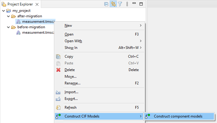
The construction process can also be configured through the same options that are available for the command-line interface. These can be configured in the dialog that is shown.

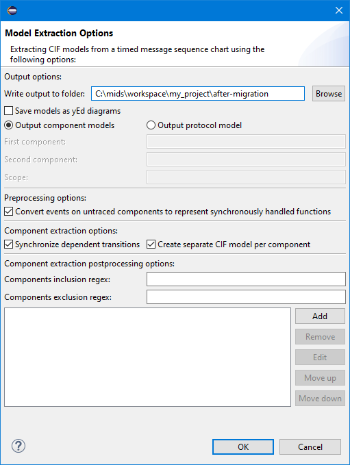
A separate dialog is available to configure post-processing operations.

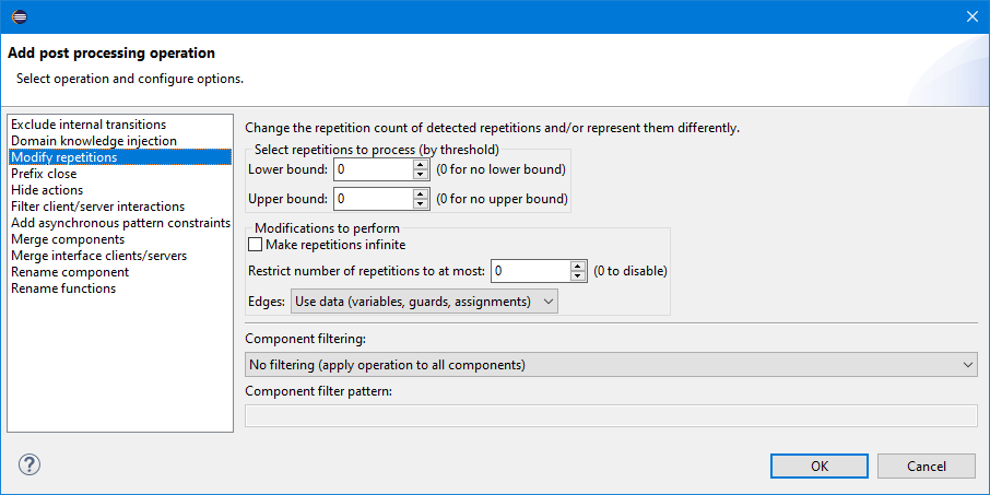
In case a sequence of operations is defined where the preconditions of an operation are not met, or one operation directly affects or removes features added by another, warnings will be given. Note that the warnings are computed statically, and since post-processing operations may be applied to only some of the components, some warnings may be false positive.

3.4. Model inference report

Constructive Model Inference produces a file component_extraction_report.txt containing a brief report of the model inference process. This file for example includes the running time of the model inference process.

3.5. Repeat inference process

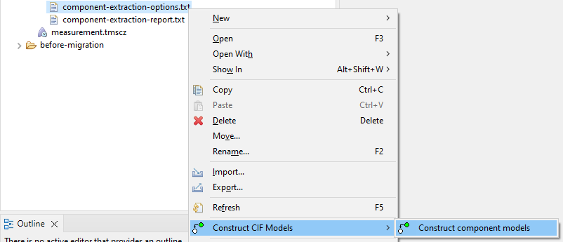
Constructive Model Inference produces a component-extraction-options.txt file as part of its output. This file can be used to repeat the inference with the same settings. Right click the options file, select Construct CIF models and then choose Construct component models.

4. Change impact analysis

To reduce risks for software evolution it is important to understand (the impact of) software changes. By comparing the software behavior before and after a redesign or patch, one can classify these changes as expected (qualified) and unexpected (regression). This way, identified regressions can be addressed early, improving confidence in the new software, reducing risks.

MIDS allows automatically comparing software behavior models. Starting at a high abstraction level, differences of interest can be inspected in more detail at lower abstraction levels, by moving through the six levels of the comparison results. Each step is supported by visualizations that allow engineers and architects to easily find (un)expected differences.

MIDS can perform a behavioral comparison of multiple sets of models. For instance, a model set for behavior before a software change (e.g. redesign, patch) can be compared to a model set capturing the behavior after the software change. Another example is comparing the software behavior for difference products being produced during a single system execution.

4.1. Preparing for comparison

A set of models consists of one or more CIF models in a directory. Multiple directories, each being a model set, can be compared.

The input models may contain (some) data depending on the model type, which is indicated by the Model type option as explained below in the next section. General CIF models (indicated by the CIF model type) are allowed to contain discrete variables. CMI models (indicated by the CMI model type) on the other hand may not contain any discrete variables other than the ones introduced by ModifyRepetitions. In particular this means that variables added by AddAsynchronousPatternConstraints post-processing are unsupported for CMI models.

The name of a model set directory serves as the name of the model set. A directory can be renamed by right clicking on it and selecting Refactor and then Rename…. Multiple directories can be given similar names by selecting all of them and choosing Bulk Rename….

4.2. Starting a comparison

In order to perform a compare, you can use the mids-compare command-line tool.

The compare tool has a number of configurable options. The tool provides a list of available options if used with the -h or -help option.

The first parameter configures which data should be compared. Providing the input path is required for every compare tool run.

Input folder (-i or -input): An input folder must be selected that contains the model sets to be compared.

This means the basic command to run the compare tool is mids-compare -i some-folder/input-data or mids-compare -input some-folder/input-data. If the output folder of the tool is not configured, the folder some-folder/output/ will be used to store the results of the comparison. This folder will be created if it does not already exist, and will be emptied if it does already exist.

To customize the compare process and the output, a number of other options are available. The other available options are:

Output folder (-o or -output)

An output folder can be selected that will contain the results of the comparison. Specify this option to override the default output folder location. It is not allowed to specify an output folder that is contained in the input folder.

Model type (-t or -type)

The type of models that are taken as input for Change Impact Analysis. Available types that can be selected are CMI and CIF. By default the input is set to CMI, i.e. the models produced by Constructive Model Inference. However, any set of CIF models can be taken as input, including ones that are not produced by CMI. Select CIF as model type for this. The entire CIF specification is considered a single entity to compare against the other CIF models. There is currently no option to compare for instance each automaton separately.

CMI compare mode (-m or -mode)

If the selected model type is CMI, the compare mode can be selected from automatic, components, protocols or service-fragments. By default automatic mode is used. Automatic mode compares service fragments of components, protocols, or entire components, depending on what is present. To compare components, the CMI option Save single model (-s or -single-model) should not be used, as comparing CIF models with multiple components is not supported. However, comparing service fragments from multiple components is supported. When a compare mode other than automatic is chosen, the input models will be compared according to the chosen mode if possible. If the selected model type is CIF, the value of this option will be ignored.

Entity type (-e or -entity-type)

The type of entity that is represented by the models. This affects only how the entities are referenced in error messages and output files. The entity type can be provided as the name of a singular entity, or as the singular and the plural form separated by a comma. The tool assumes the provided entity type is lower case and will change the first character to upper case as needed. If the chosen entity type should always be written with an upper case first character, it should be provided as such. Additionally, if no plural is provided, s is appended to the singular form to create the plural. Both singular and plural names may contain any character except commas. For example, entity type can be configured as component or entity,entities. If no entity type is selected using this option, an entity type will be selected by the tool. When the model type is CIF, the entity type chosen is always entity. When the model type is CMI, the entity type corresponds to the model type.

Color scheme (-c or -color)

The output of the comparison will include a matrix that shows differences between model sets (more on that later, in the upcoming section about compare output, on level 3). This matrix uses colors to highlight any parts with significant differences. This options configures the matrix color scheme to use. Available choices are intuitive and large-range, where intuitive is the default selection. The intuitive color scheme uses a reduced range of colors selected to best match intuition. The reduced range does result in the disadvantage that small differences can be hard to discern, because the colors used are very similar. The large range color scheme addresses this issue by using a larger range of colors, making it possible to separate values more, at the cost of using less intuitive colors.

Skip post-processing level 6 compare results (-p or -no-post-process)

By default, the difference state machines shown in level 6 are post-processed to increase their readability. Intuitively, post-processing searches for state-machine patterns that may be simplified. Enabling this option will disable such post-processing, which may improve performance but may also reduce the quality of the compare results.

Compare algorithm (-a or -algorithm)

The calculation of difference state machines involves comparing the structures of two state machines and determining their difference. More details will be provided in the upcoming section about compare output, on level 6. There are several algorithms available for doing these comparisons. The different available algorithms make a trade-off between computational intensity and quality of the results:

The heavyweight algorithm outputs a high-quality result, but requires a lot of computational resources. This algorithm is only recommended when the input models are relatively small (say, less than 50 states each).
The lightweight algorithm is much cheaper in terms of computational intensity, at the cost of quality. This algorithm is recommended when the input models are mostly large.
The dynamic algorithm applies either the lightweight or the heavyweight algorithm, depending on the sizes of each individual comparison. This algorithm is recommended if the input models are a mix of both small and large input models.
The walkinshaw algorithm applies the algorithms by Walkinshaw. It is between the lightweight and heavyweight algorithms in terms of computational intensity and quality.
The bruteforce algorithm give an optimal result that is sometimes better than the results of the heavyweight algorithm. But it is also much more computationally intensive (in the worst case) since it explores all the possible ways in which the differences between two state machines can be represented, to select the minimal one.

The default algorithm selected is dynamic.

Extend lattice (-x or -extend-lattice)

During the computation of the level 2 and level 5 lattices, the compare tool can compute models and model sets to complete the lattices. This option can be used to configure that behavior, by using the argument none, partial or full. By default or if the argument partial is chosen, lattices are completed but the computed model sets and models are only shown in levels 2 and 5 respectively. If the argument none is chosen, the lattices are not completed and no computed models or model sets are present in any level. In contrast, if the argument full is chosen, lattices are completed and the computed models and model sets are shown in all levels. Note that the union/intersection size limit option can be used to further configure lattice completion.

SVG generation timeout in seconds (-ts or -timeout-svg)

The comparison process will generate SVG files. This option configures the timeout (in seconds) for generating such files. If generation takes longer than the configured value, it will be halted and a warning will be produced to indicate the problem. The default value of the timeout is 60 seconds.

Union/intersection size limit (-l5 or -size-limit-level5)

The compare process calculates additional ('computed') model variants from existing model variants using state machine union and intersection operations. This option indicates the maximum size of models (measured in number of states) to be considered for union and intersection computations. The default value for the union/intersection size limit is 100 states. Models that have more states will not considered for union and intersection. As this may lead to incomplete information, this is presented differently in levels 2 and 5 (see below). If the option for extending lattices is used with the argument none, the value set for this option is not used.

Structural compare size limit (-l6 or -size-limit-level6)

This option indicates the maximum size of models (measured in number of states) to be considered for structural comparison. Models that have more states will not be structurally compared. This may lead to incomplete information in levels 5 and 6 (see below). The default value for the structural compare size limit is 5000 states.

Options file (-f or -options-file)

In addition to command line options, settings can be provided in an options file. An options file should be a text file contain one or more compare tool options. Each option and each argument should be on a separate line. As an exception, the options file option itself will be ignored if used in an options file. At the end of each run, the compare tool produces a compare-options.txt file containing the settings for that run, which can be used to repeat the run. Option values defined on the command line take precedence over values defined in the options file.

4.2.1. Comparison in the MIDS UI

In order to perform a compare in the MIDS UI, you can use the right click Compare CIF models action in the MIDS UI on a directory that contains all model sets that should be compared.

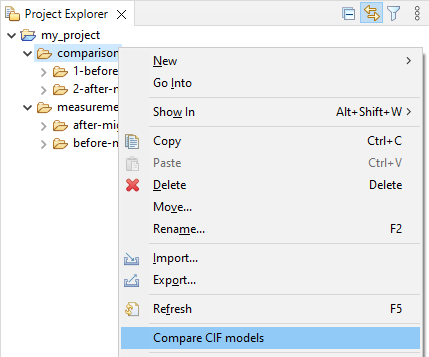
This action will show a dialog with configuration options for the comparison.

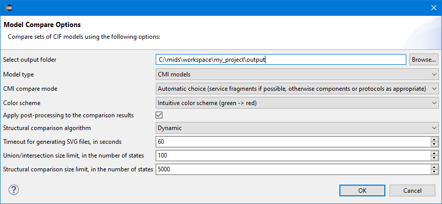
The available options are the same as for the command-line tool.

4.3. Compare output

The output of the compare tool is centered around the index.html file.

When performing a compare in the MIDS UI, it is recommended to use a modern external browser to view the index.html file, as the browser integrated in the MIDS tooling is outdated and limited in functionality.

This file contains an overview of the comparison results, presented as six different levels. The first three focus on model sets, while the last three focus on individual models within the model sets. For both model sets and models, there are three levels: variants, variant relations and variant differences.

For readability purposes, in the following text, we will assume the items compared are entities. Wherever entities are mentioned, the same also applies to other entity types such as components or service fragments.

By default, CMI produces a model per entity, either as a single file or as a file per entity. In either case the compare tool will consider entity models, and model sets will contain models for different entities.

If the input models contain component models that consist of service fragments, these will be split if the chosen compare mode is service-fragments or automatic. In that case the compare tool will consider service fragment models, and model sets will contain models for service fragments of different components. Effectively, this increases the level of detail of the compare output, as differences are shown per service fragment, i.e. a part of a component, rather than for the whole component.

Below each of the six levels is explained in more detail.

4.3.1. Level 1: Model set variants

At the highest level, we look at differences between entire model sets.

This level shows which model sets are equal to which other model sets, as indicated by model set variants. Two model sets that have the same variant contain the same behavior for all entities, while two model sets with different variants have at least one difference in entity behavior.

This is primarily relevant when comparing a larger number of model sets that each represent an instance of a repeated process, because it shows which model sets contain exceptional behavior. This level allows to get an overview of the model sets and their behavior, and identify patterns over the various model sets.

4.3.2. Level 2: Model set variant relations

In the next level, we look at the relations between the model set variants that have been identified.

In particular, we observe some model sets may contain behavior that is an extension of the behavior in another model set. By connecting model set variants that have this relation, we can create a (partial) lattice of variants. An arrow from one model set variant to another indicates that the behavior of the first model set variant is completely contained in the latter model set variant, i.e. the latter extends the former.

Additionally, we can compute additional ('computed') model set variants such that the lattice is completed. These computed model sets are indicated in the lattice by diamond shapes, while variants based on input model sets are indicated by ellipses.

On the edges between the model set variants, the size of the difference is shown as the number of added entities (e.g. +5 in green) and changed entities (e.g. ~5 in blue).

This level allows to relate the model set variants to each other, to determine which to investigate in more detail.

Model set variants that contain models that are too large (see the Union/intersection size limit option) will not be related to the other model set variants. Their shapes get a dashed border to indicate incomplete information.

4.3.3. Level 3: Model set variant differences

The third level shows a more detailed view of the differences between model sets, in the form of a matrix that shows for each model set pair how many entities are different between them. The cells of the matrix are colored based on the number of differences, to better emphasize where significant similarities and differences can be found.

This level allows to find patterns on the behavior of larger amounts of model sets.

4.3.4. Level 4: Model variants

In this level, we look at differences in the behavior of entities in different model sets. The differences are displayed as a table showing for each combination of entity and model set which variant of the entity, if any, is present in the model set. By comparing the entity behavior variants present in various model sets, we can identify which model sets have different behavior for that entity and how many variants there are.

This level allows to find out which entities have different behavior at all. It also allows to find patterns on the behavior of an entity over the different model sets.

One can click on any variant in the table to see the state machine model corresponding to that variant.

4.3.5. Level 5: Model variant relations

In this level, the relations between the behavioral variants of entities are shown.

Entity variants are considered related when the behavior of one variant is an extension of the behavior of another. By connecting entity variants that have this relation, we can create a (partial) lattice of variants. An arrow from one entity variant to another indicates that the behavior of the first entity variant is completely contained in the latter entity variant, i.e. the latter extends the former.

Additionally, we can compute additional ('computed') entity variants such that the lattice is completed. These computed entity variants are indicated in the lattice by diamond shapes, while variants based on input entity variants are indicated by ellipses.

On the edges between the model variants, the size of the difference is shown as the number of added transitions (e.g. +5 in green) and removed transitions (e.g. -5 in red). The Structural compare size limit option may limit the computation of structural differences, leading to a lack of information. If the information is not computed, a question mark (?) is shown on the edge instead.

This level allows to relate the variants of an entity to each other, to determine which to investigate in more detail.

Model variants that are too large (see the Union/intersection size limit option) will not be related to the other model variants. Their shapes get a dashed border to indicate incomplete information.

4.3.6. Level 6: Model variant differences

This level shows the differences between specific entity variants. These variants are presented in a table, and one can click on diff to see the differences between two variants indicated by the row and column of the table.

The differences are represented using a state machine view of the model. In this view, one of the variants serves as a base (the one indicated in the row of the table), and coloring indicates where states and transitions have to be added, changed or removed to reach the second variant (the one indicated in the column of the table). Clicking on an edge in the state machine opens a side panel containing additional information about that edge. The panel can be closed by using the close button in the top right corner, or by clicking the edge again.

Depending on the comparison settings, differences are available only between variants directly related in the variant lattice (level 5), or additionally between all input variants. The Structural compare size limit option may limit the computation of structural differences, leading to some comparisons being skipped and their results not being available.

5. Release Notes

The release notes of the Model Inference and Differencing Suite (MIDS) are listed below, in reverse chronological order.

5.1. MIDS v1.0

The first open-source release of MIDS.

5.2. MIDS v0.1 to v0.9

Release notes of older version of MIDS are no longer available.